

In an age where computing power surrounds us, it’s easy to become wrapped up in the idea that information is processed and delivered like magic; so fast that we sometimes forget that millions of calculations per second are being done between the time we requested the information and the time it is delivered.
While it’s true that machine computation time is taken for granted, on a more granular scale, all work still requires time. And when the work-load begins to mount, it becomes important to understand how the complexity of an algorithm influences the time it takes to complete a task.
An algorithm is a step-by-step list of instructions used to perform an ultimate task. A good software engineer will consider time complexity when planning their program. From the start, an engineer should consider a scenario that their program may encounter that would require the most time to complete if at all. This is known as the worst-case time complexity of an algorithm. Starting from here and working backwards allows the engineer to form a plan that gets the most work done in the shortest amount of time.
Big O notation is the most common metric for calculating time complexity. It describes the execution time of a task in relation to the number of steps required to complete it.
Big O notation is written in the form of O(n) where O stands for “order of magnitude” and n represents what we’re comparing the complexity of a task against. A task can be handled using one of many algorithms, each of varying complexity and scalability over time.
There are myriad types of complexity, the more complicated of which are beyond the scope of this post. The following, however, are a few of the more basic types and the O notation that represent them. For the sake of clarity, let’s assume the examples below are executed in a vacuum, eliminating background processes (e.g. checking for email).
Constant Complexity: O(1)
A constant task’s run time won’t change no matter what the input value is. Consider a function that prints a value in an array.
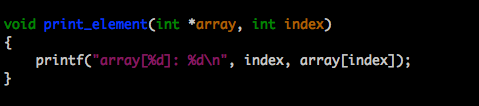
No matter which element’s value you’re asking the function to print, only one step is required. So we can say the function runs in O(1) time; its run-time does not increase. Its order of magnitude is always 1.
Linear Complexity: O(n)
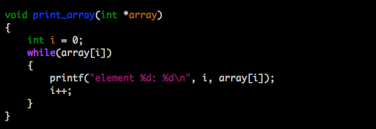
A linear task’s run time will vary depending on it’s input value. If you ask a function to print all the items in a 10-element array, it will require less steps to complete than it would a 10,000 element array. This is said to run at O(n); it’s run time increases at an order of magnitude proportional to n.
Quadratic Complexity: O(N²)
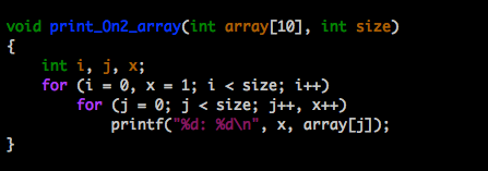
A quadratic task requires a number of steps equal to the squaure of it’s input value. Lets look at a function that takes an array and N as it’s input values where N is the number of values in the array. If I use a nested loop both of which use N as it’s limit condition, and I ask the function to print the array’s contents, the function will perform N rounds, each round printing N lines for a total of N² print steps.
Let’s look at that practically. Assume the index length N of an array is 10. If the function prints the contents of it’s array in a nested-loop, it will perform 10 rounds, each round printing 10 lines for a total of 100 print steps. This is said to run in O(N²) time; it’s total run time increases at an order of magnitude proportional to N².
Exponential: O(2^N)
O(2^N) is just one example of exponential growth (among O(3^n), O(4^N), etc.). Time complexity at an exponential rate means that with each step the function performs, it’s subsequent step will take longer by an order of magnitude equivalent to a factor of N. For instance, with a function whose step-time doubles with each subsequent step, it is said to have a complexity of O(2^N). A function whose step-time triples with each iteration is said to have a complexity of O(3^N) and so on.
Logarithmic Complexity: O(log n)
This is the type of algorithm that makes computation blazingly fast. Instead of increasing the time it takes to perform each subsequent step, the time is decreased at magnitude inversely proportional to N.
Let’s say we want to search a database for a particular number. In thedata set below, we want to search 20 numbers for the number 100. In this example, searching through 20 numbers is a non-issue. But imagine we’re dealing with data sets that store millions of users’ profile information. Searching through each index value from beginning to end would be ridiculously inefficient. Especially if it had to be done multiple times.
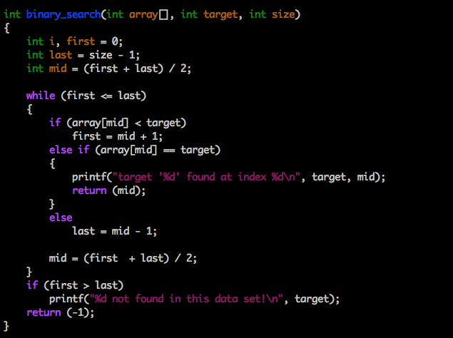
A logarithmic algorithm that performs a binary search looks through only half of an increasingly smaller data set per step.
Assume we have an asscending ordered set of numbers. The algorithim starts by searching half of the entire data set. If it doesn’t find the number, it discards the set just checked and then searches half of the remaining set of numbers.
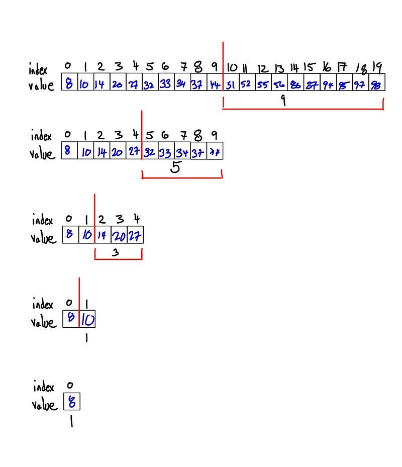
As illustrated above, each round of searching consists of a smaller data set than the previous, decreasing the time each subsequent round is performed. This makes log n algorithms very scalable.
While I’ve only touched on the basics of time complexity and Big O notation, this should get you off to a good start. Besides the benefit of being more adept at scaling programs efficiently, understanding the concept of time complexity is HUGE benefit as I’ve been told by a few people that it comes up in interviews a lot.


